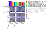
Preprint Initial findings from the DecodeME genome-wide association study of myalgic encephalomyelitis/chronic fatigue syndrome, 2025, DecodeMe Collaboration

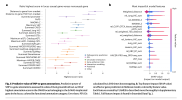
Is what's causing PEM activity of the brain in excess of what it can tolerate due to some problem at the synapses?

Is there any indication that glutaminergic synapses are playing a role in ME/CFS?

What's the similarity between autism and ME/CFS?
 
Like @forestglip and @ME/CFS Science Blog I’ve spent some time digging into some tools including magma/fuma and annovar. And learnt a bit about the myriad hurdles and technical issues bioinformatics students and researchers must live with. After a week much of my understanding is likely way off but I have a few questions, maybe they’re best for @Chris Ponting and the authors but perhaps others with more experience can chime in?

Were the GWAS summary statistics (hg38) or other/raw data used for MAGMA/FUMA analysis? What reference panel was used? These tools and the default panels seem to depend upon different human genome versions/reference assemblies than hg38, was liftover used or re-calling? I’m unsure about some other settings like the window size too, which could effect things quite a lot.

Knowing more about the methods, data and settings here would help reproducibility and understanding I think. And I wonder about what risks/loss there are with conversions between formats?

This study used an additive model I think, would it be worth exploring results from recessive/dominant models too?

I have learned new words like exonic, intronic and intergenic and as far as I can tell most findings (88%) from GWAS studies are in these interonic and intergenic regions. Although these don’t directly change the protein, it seems they can modify things a lot by effecting expression through things like translation.

There seems lots of scope for more analysis here, understanding what is in LD with the identified SNPs and using more tools like annotation to help get an idea of potential mechanisms. Or did the eQTL and risk loci cover this? I’ve not started looking at that yet and don’t understand the pros/cons of different methods.

Is this sort of wider analysis planned? Is the hope others may take it up? Would it be possible to make more of the data available to help others do this?

A bit of a mishmash of questions and thoughts….
 
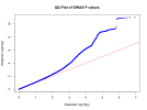
Don't think we have discussed this plot yet:
1755695341674.png
Basically, the idea is that if the difference between groups is driven by selection bias, stratification effects, ancestry differences etc., then there will be lower p-values across the board. It would look like a systematic shift where many SNPs are affected, too many to be explained by genetic differences underlying a disease.

A true effect of the genetic susceptibility for a disease should result in a smaller number of SNPs that are significantly different.

One way to test and differentiate between the two is to plot the p-values found against a uniform distribution of p-values (because that's what we would expect if there was no effect). If we're testing the genetics of the disease, then we would see the observed p-values differ from the expected, only at the very end, like a tail that bends upward. If there were a systematic difference, then the observed and expected would not match for many other p-values, and so the straight line would break and bend earlier. It would not match a straight line through the origin with a slope of 1.

I have little experience with interpreting these plots, but it looks like there was some systematic difference for the low allele frequencies and no or much less for the common frequencies, which is where most of the hits were found. Because the observed p-values go all the way up to 10^-11, I assume this shows the full data before filtering based on quality control took place? EDIT: see comment from forestglip below.

There is also an inflation measure, lambda = 1.066, which is the ratio of the observed to expected median p-value. Here, the same reasoning applies: these should be similar (so lambda should be close to 1). If not, it would suggest population differences other than having ME/CFS or not. A lambda of 1.066 looks fine.
 
Last edited:
Like @forestglip and @ME/CFS Science Blog I’ve spent some time digging into some tools including magma/fuma and annovar. And learnt a bit about the myriad hurdles and technical issues bioinformatics students and researchers must live with. After a week much of my understanding is likely way off but I have a few questions, maybe they’re best for @Chris Ponting and the authors but perhaps others with more experience can chime in?

Were the GWAS summary statistics (hg38) or other/raw data used for MAGMA/FUMA analysis? What reference panel was used? These tools and the default panels seem to depend upon different human genome versions/reference assemblies than hg38, was liftover used or re-calling? I’m unsure about some other settings like the window size too, which could effect things quite a lot.

Knowing more about the methods, data and settings here would help reproducibility and understanding I think. And I wonder about what risks/loss there are with conversions between formats?

This study used an additive model I think, would it be worth exploring results from recessive/dominant models too?

I have learned new words like exonic, intronic and intergenic and as far as I can tell most findings (88%) from GWAS studies are in these interonic and intergenic regions. Although these don’t directly change the protein, it seems they can modify things a lot by effecting expression through things like translation.

There seems lots of scope for more analysis here, understanding what is in LD with the identified SNPs and using more tools like annotation to help get an idea of potential mechanisms. Or did the eQTL and risk loci cover this? I’ve not started looking at that yet and don’t understand the pros/cons of different methods.

Is this sort of wider analysis planned? Is the hope others may take it up? Would it be possible to make more of the data available to help others do this?

A bit of a mishmash of questions and thoughts….
Hi. Yes, we needed to LiftOver DNA variants from human genome build 38 (hg38) to the previous version (GRCh37 (hg19)) which FUMA uses for, e.g., MAGMA analysis. You're correct that some SNPs are lost in the LiftOver, but only a few. More variants are lost because FUMA's reference panel of variants is incomplete. Yes, the GWAS model we used in REGENIE is an additive linear model. But we are also applying non-additive, non-linear models separately (TarGene; will report when we have results). Yes - as with nearly all GWAS - are lead SNPs are not in protein-coding sequence. And, yes, there is scope for a lot more analyses both by us (DecodeME) and any researchers who receive the consented and pseudoanonymised data via the Data Access Committee. The preprint's title starts with "Initial Results..." and we mean this. Yet more to come.
 
Last edited:
Thanks @Chris Ponting I look forward to seeing what more there is to come and echo @Hoopoe in thanking you and the rest of the team, for all you’ve done so far. The more I’m learning the more possibilities and scope there seems to be, exciting times!

Really useful answers in general but also in helping my understanding of the process. I wasn’t sure if I’d just missed something wrt FUMA/MAGMA (it also seems they briefly supported hg38 but now don’t).

I’ve just finished running magma 1.10 standalone from the command-line on gwas-1 using hg38 (amazing what you can do on a raspberry pi!). Although tbh it’s difficult to know what else I may have missed or got wrong in the process and it uses the same reference data (https://cncr.nl/research/magma/) so may have the same problems. But I’ll try to write up my steps so others here can have a prod at it.
 
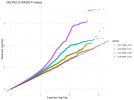
Ah yes apologies. I think I'm a bit confused because those low p-values shown in the graph are in purple and for the category: 0.01 ≤ MAF < 0.04, but I thought that the hits found had MAF > 10%?
Oh good point. If I'm understanding correctly, the furthest right, uppermost dot is 20:48914387:T:TA (the lead hit in the whole study), but its MAF is around .34.
 
Hi. Yes, we needed to LiftOver DNA variants from human genome build 38 (hg38) to the previous version (GRCh37 (hg19)) which FUMA uses for, e.g., MAGMA analysis. You're correct that some SNPs are lost in the LiftOver, but only a few. More variants are lost because FUMA's reference panel of variants is incomplete. Yes, the GWAS model we used in REGENIE is an additive linear model. But we are also applying non-additive, non-linear models separately (TarGene; will report when we have results). Yes - as with nearly all GWAS - are lead SNPs are not in protein-coding sequence. And, yes, there is scope for a lot more analyses both by us (DecodeME) and any researchers who receive the consented and pseudoanonymised data via the Data Access Committee. The preprint's title starts with "Initial Results..." and we mean this. Yet more to come.
Hi Chris, sincere thanks for all your hard work and advocacy on our behalf. Exciting to hear more analyses of the data are in the works!

I was wondering if there was any sort of timeframe for the publication of the HLA analysis? And am curious whether the Manhattan plot published with the initial data shows the HLA data points or whether they were removed from the plot whilst the analysis is ongoing?
No timeframe for completion of the HLA analysis. The Manhattan plot in the preprint includes all variants including those in the HLA. But note that in the HLA analyses we do not test each DNA variant, rather we test combinations of variants that are commonly coinherited, i.e. "HLA alleles". So even if there isn't a "signal" in the Manhattan plot this does not immediately mean that we won't see association to an HLA allele.
 
Don't think we have discussed this plot yet:
Tried to recreate the plot using the whole dataset:

1755798455731.png

I thought it started to deviate from the red line (which has a slope of 1) quite soon already from an observed -log10 p-value of 3. But the graph is a bit misleading because it is logarithmic so the vast majority of points are in the region to the left of this (there are so many points that you can't see the difference). For example more than 90% of points have an observed -log10 p-value < 4.

So it's mostly the bottom left region of the graph that matters for interpreting inflation, and that seems to close to the red line.
 
Oh good point. If I'm understanding correctly, the furthest right, uppermost dot is 20:48914387:T:TA (the lead hit in the whole study), but its MAF is around .34.
Looks like a labelling issue of the graph. Here's what I got trying to recreate it. The high p-values belong to the SNPs with high MAF values, showing that it was mostly this group that reached significant hits.

@Chris Ponting

1755805502894.png
 
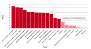
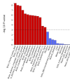
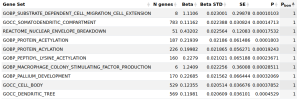
As mentioned above, something @forestglip and I have been working on recently is running MAGMA locally on the DecodeME summary statistics.

I wouldn’t necessarily recommend anyone do this or follow these instructions. There may be things wrong with this method and it seems to end up with only 94% of variants mapped while @forestglip gets over 99% using the LiftOver and FUMA method mentioned earlier.

But it was a useful exercise to learn a bit about the process and in sharing this we hope others can learn or indeed point out errors, which helps us learn!

A recipe for gene enrichment with DecodeMe and MAGMA
You will need the following ingredients
- a computer with a shell (performed on Linux but can also be done on Mac or Windows)​
- an understanding of installing and running tools from command-line​
enough space to download lots of data (15GB or so)​

Prepare your tools
- As well as standard tools like awk and zcat you will need to install sort-bed, bedmap and magma itself​
- Magma binaries and source for yourself are available from https://cncr.nl/research/magma/
- The apt package bedops provides sort-bed and bedmap or for more info https://github.com/bedops/bedops

Prepare your data
- DecodeME summary stats files and the list of variants that passed qc are available here https://osf.io/rgqs3/files/osfstorage
- You will also need gene locations (build38) and reference data (European) from here https://cncr.nl/research/magma/
- Molecular Signals Database files from https://www.gsea-msigdb.org/gsea/msigdb (the complete Human MSigDB v2025.1.Hs release, described as Human Gene Set GMT file set (ZIPped)​
- UCSC genome annotation database for GRCh38/hg38) assembly​

We recommend organising these into tools and data folders for easy management, especially if you’ll be running multiple passes with different databases or options. Most need unzipping although the snp151 database is very large so best left zipped.

Then perform the following steps

Filter the main gwas file to include just those variants which passed quality control
Code:
awk -v OFS='\t' 'FNR==NR {ids[$1]++; next} NR==1 || ($3 in ids)' gwas_qced.var gwas_1.regenie > filtered_regenie_file.txt

Add rsid information to these summary stats
First we create then sort a bed formatted file of chromosomes and positions (zero indexed) from the above
Code:
awk -v OFS='\t' 'NR!=1 { print "chr"$1, $2-1, $2, $0 }' filtered_regenie_file.txt > query.bed
sort-bed query.bed > sorted_query.bed

And filter the UCSC genome annotation database to include only single nucleotide variations and again output this in bed format
Code:
zcat snp151.txt.gz | awk -v OFS='\t' '{if($12=="single") print $2,$3,$4,$5}' > snp151_snp.bed

Then we use bedmap to matching rsids to the positions in the summary stats bed file
Code:
bedmap --echo --echo-map-id --delim '\t' sorted_query.bed snp151_snp.bed > sorted_query_with_rsids.bed

Now we prepare the data for MAGMA
First create a gene position file from the above using the rsids as an index
Code:
awk -v OFS='\t' '$21 != "" {print $21,$4,$5}' sorted_query_with_rsids.bed > decodeme.magma_input.id.chr.genpos.txt

Then a p value file
Code:
awk -v OFS='\t' '$21 != "" {print $21,10^(-$19)}' sorted_query_with_rsids.bed > decodeme.magma_input.id.p.txt

Now we can use MAGMA to annotate
Code:
snploc=./decodeme.magma_input.id.chr.genpos.txt
ncbi38=./NCBI38.gene.loc
magma --annotate \
      --snp-loc ${snploc} \
      --gene-loc ${ncbi38} \
      --out decodeme

Then perform gene based analysis
Code:
ref=./g1000_eur/g1000_eur
magma \
    --bfile $ref \
    --pval ./decodeme.magma_input.id.p.txt N=275488 \
    --gene-annot decodeme.genes.annot \
    --out decodeme

And finally gene-set analysis
Code:
geneset=msigdb_v2025.1.Hs_GMTs/c5.all.v2025.1.Hs.entrez.gmt
magma \
    --gene-results decodeme.genes.raw \
    --set-annot ${geneset} \
    --out decodeme

After a short wait you will have some delicious data to consume with friends!

Thanks to those who made and documented these tools
https://cncr.nl/research/magma/
https://bedops.readthedocs.io/en/latest/

As well the wise and informative internet for its advice on how to use them
https://cloufield.github.io/GWASTutorial/09_Gene_based_analysis/
https://hanbin973.github.io/bioinformatics/2023/02/20/rsid.html


There’s also a handy bash script attached, which will ask for paths to the relevant locations and run it all for you. This also saves configurations and allows reuse of some intermediate files so makes multiple runs with slightly different settings or data easier. The script was put together with help from Gemini Pro for all the boring scaffolding.
 

Attachments

As mentioned above, something @forestglip and I have been working on recently is running MAGMA locally on the DecodeME summary statistics.

I wouldn’t necessarily recommend anyone do this or follow these instructions. There may be things wrong with this method and it seems to end up with only 94% of variants mapped while @forestglip gets over 99% using the LiftOver and FUMA method mentioned earlier.
Thanks for delving into this!

It looks so complicated. I expected that there would be nice packages in R and Python that wrap this into a handy user interface and provide the correct reference data (for LD, for example) automatically. Quite disappointing that the workflow mostly consists of command-line instructions and extracting the right data and tools from the web.

Yesterday I tried doing the LDSC and stumbled onto one problem after the other (it only runs on Python2, need to convert GRCh38 to rsID, download the correct reference data online, etc.). I ran out of energy but hope to try again later.
 
Last edited:
Thanks for delving into this!

It looks so complicated. I expected that there would be nice packages in R and Python that wrap this into a handy user interface and provide the correct reference data (for LD, for example) automatically. Quite disappointing that the workflow mostly consists of command-line instructions and extracting the right data and tools from the web.

Yesterday I tried doing the LDSC and stumbled into one problem after the other (it only runs on Python2, need to convert GRCh38 to rsID, download the correct reference data online, etc.). I ran out of energy but hope to try again later.
Unfortunately a lot of bioinformatics pipelines are pretty hodgepodge and you need to be a Jack of all trades to get something new up and running. It’s true that all of coding is 90% troubleshooting, but for bioinformatics especially where almost none of the packages/tools were designed by people explicitly trained in software engineering, it can be hell in a handbasket with entire weeks wasted. I started out in research with only a little bit of self-taught R experience and immediately got thrown headfirst into trying to understand what awk was with no help except stack exchange—I’m glad I had already developed the ability to parse through complete gibberish and not get overwhelmed, otherwise it would have discouraged me from science all together.

Nextflow has improved things somewhat—it’s a crowdsourced automated pipeline collection that basically handles all the intermediate steps for you. But when something breaks or if you need to customize anything, it’s a nightmare and a half. And you’re limited to the few highly used pipelines that have been developed and tested by a kind soul.

Huge props to folks on this thread for diving right into it and being so quick on the uptake!
 
It looks so complicated. I expected that there would be nice packages in R and Python that wrap this into a handy user interface and provide the correct reference data (for LD, for example) automatically.
Note that the script hotblack posted includes a lot of extras for convenience, like remembering settings for future runs. These are the only required steps we used:
Bash:
# First store all variants from gwas_qced.var in ids array.
# Then loop over every row in gwas_1.regenie and save to filtered_regenie_file.txt if it's the first row (header) or if the third column (the ID) is in the ids array.
awk 'FNR==NR {ids[$1]++; next} NR==1 || ($3 in ids)' gwas_qced.var gwas_1.regenie > filtered_regenie_file.txt

# For all but first row, print the chromosome, position-1, position, and entire original line to query.bed
# Need to subtract one because .bed files are zero indexed
awk 'NR!=1 { print "chr"$1, $2-1, $2, $0 }' filtered_regenie_file.txt > query.bed

# Sort bed file
sort-bed query.bed > sorted_query.bed

# Filter rsid reference file to only include SNVs.
# Pipe decompressed file to awk
# Set output separator to tab
# If the twelfth column is "single" (SNV), output chr, pos, pos, rsid (bed format)
zcat snp151.txt.gz | awk -v OFS='\t' '{if($12=="single") print $2,$3,$4,$5}' > snp151_snp.bed

# Add matching rs ids to the positions in the summary stats bed file
bedmap --echo --echo-map-id --delim '\t' sorted_query.bed snp151_snp.bed > sorted_query_with_rsids.bed

# Create SNP position file from summary statistics for MAGMA
# The format is 'rsid    chromosome    position'
awk '$21 != "" {print $21,$4,$5}' sorted_query_with_rsids.bed > decodeme.magma_input.id.chr.genpos.txt

# Create SNP p value file from summary statistics for MAGMA
# The format is 'rsid    p-value'
awk '$21 != "" {print $21,10^(-$19)}' sorted_query_with_rsids.bed > decodeme.magma_input.id.p.txt

# Annotate genes with SNPs
snploc=./decodeme.magma_input.id.chr.genpos.txt
ncbi38=./NCBI38.gene.loc
magma --annotate \
      --snp-loc ${snploc} \
      --gene-loc ${ncbi38} \
      --out decodeme

# Do gene-based analysis to create score for each gene
ref=./g1000_eur/g1000_eur
magma \
    --bfile $ref \
    --pval ./decodeme.magma_input.id.p.txt N=275488 \
    --gene-annot decodeme.genes.annot \
    --out decodeme

# Run gene-set analysis
geneset=msigdb_v2025.1.Hs_GMTs/c5.all.v2025.1.Hs.entrez.gmt
magma \
    --gene-results decodeme.genes.raw \
    --set-annot ${geneset} \
    --out decodeme

FUMA does make MAGMA much easier (though requires converting to GRCh37). I've been looking for other online tools for analyzing GWAS data. The following each have several other automatic analysis tools where you mainly just need to upload the summary stats (though unfortunately you do need the data to have rs ids for at least the second website), though I haven't tried any of the tools yet. The second one looks like it has LDSC.

SysBiol PostGWAS

Complex-Traits Genetics Virtual Lab

The main struggle seems to be either mapping the variants to rs ids or converting from GRCh38 to GRCh37, and it doesn't seem that either is a trivial task to do exactly right. I'm not sure we did the rs id mapping perfectly since we based it only on positions and not letters. Surprisingly hard to find good explanations.

Edit: Also we found later that "single" in the rsid reference file doesn't only mean SNVs. I think it includes all single letter insertions or deletions as well, so not sure how that affects things.
 
Last edited:
Back
Top Bottom